Foresight Technical Deep Dive
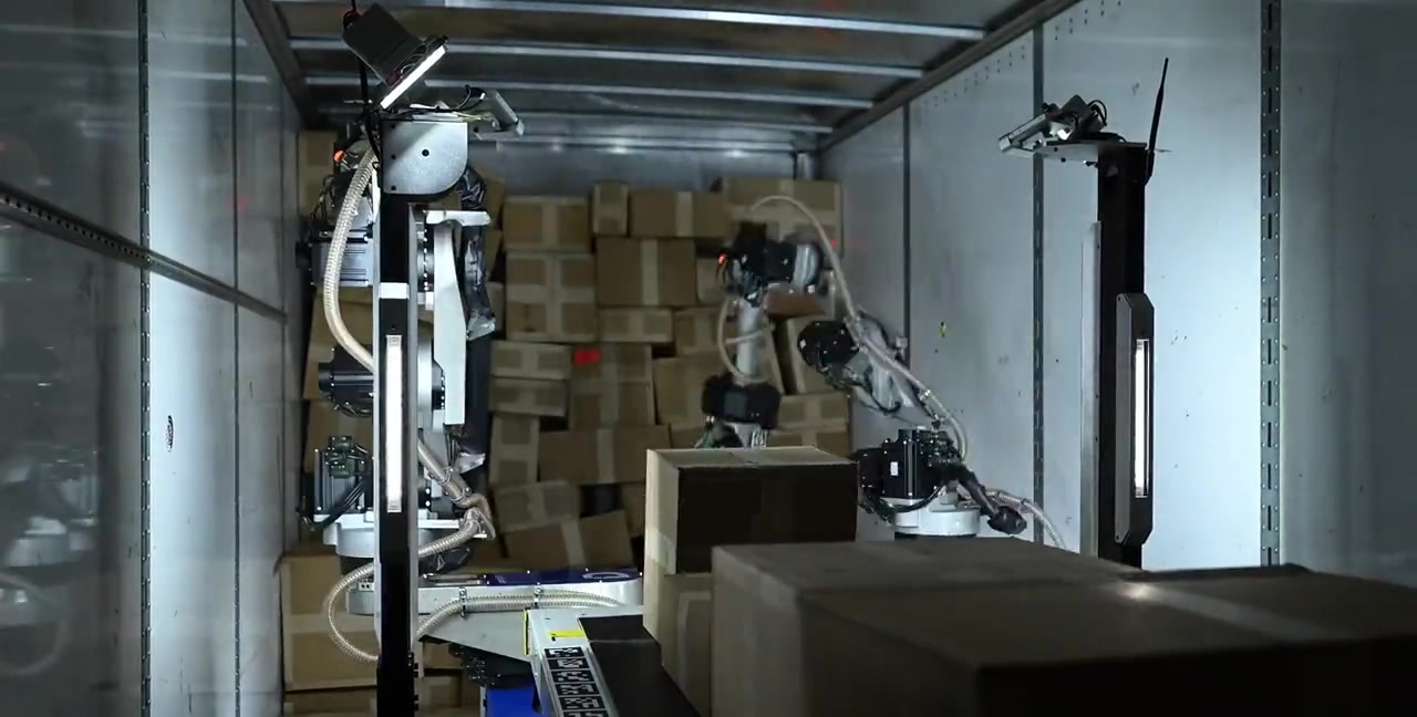
Inside Foresight: From Packing Evaluation to Real-Time Coordination
How we measure a production packing agent's planning intelligence — and how predictive pipelining turns those plans into highly-parallelized packing across two robot arms in production.
Density
0.68
Parallelism
72%
Pipelining
65.5%
Retry Required
0.18%
In Introducing Foresight, we described what Foresight does. This companion post is about how we know it works — and how we measure its impact.
Part I covers the Foresight-powered packing agent — the planning intelligence that decides where every box goes. Part II covers the Foresight-powered execution layer — the real-time coordination that turns those plans into 400+ picks per hour across two robot arms.
These aren’t cherry-picked results. They’re the systematic evaluations and production measurements we use internally to make deployment decisions.
Part I
Planning Intelligence
Building a packing agent that works in simulation is hard. Building one that works in production — under real-time constraints, with imperfect perception, on a physical robot — is a different problem entirely. Foresight powers a packing agent that jointly optimizes density, stability, and throughput. These six sections cover how we evaluate it: the metrics, the statistics, and the tradeoffs.
01
Baseline Performance Across Distributions
We evaluated Foresight on four distinct box distributions drawn from real warehouse data. Each brings a different mix of box sizes, weights, and shapes. These results represent the agent simultaneously optimizing for all objectives — density, stability, throughput, and placement quality — in a realistic physics environment with robot kinematic constraints and gripper force limits.
What is a sequence?
Each sequence is a single evaluation episode: the packing agent fills a ~2-meter-long section of a trailer with boxes drawn one at a time from a real-world distribution. The agent sees only the current box and the state of the trailer — no lookahead.
We evaluate under two constraint regimes. Full robot constraints enforce kinematic reachability, gripper force limits, and dual-arm collision avoidance — the conditions the agent actually faces in production. Light robot constraints relax reachability checks to isolate algorithmic packing quality from robot-specific penalties, giving us a useful calibration baseline. The gap between regimes quantifies the cost of production constraints — or conversely, the benefit we stand to gain if we can lift them.
| Metric | Description |
|---|---|
| Densityprimary | Ratio of total box volume to the bounding region volume across completed walls. Measures how efficiently the agent fills the available trailer space. |
| Parallelismprimary | Fraction of consecutive placements that could execute simultaneously on two robot arms. |
| Stabilityprimary | Fraction of sequences without any structural failure or collapse. Small shifts/tilts of boxes are acceptable. |
| Tilt | Average angular deviation (in degrees) of each box's up-axis from vertical, after physics settlement. |
| Fissures | Total gap area (in m²) in the wall cross-section up to 1 meter height, summed across completed walls. |
| Dataset | Constraints | Density | Parallelism | Stability | Tilt (°) | Fissures (m²) |
|---|---|---|---|---|---|---|
| Distribution A | Full | 0.72 [0.72, 0.73] | 66% [0.64, 0.67] | 100% [99.52, 100] | 2.37 [2.27, 2.50] | 0.62 [0.61, 0.66] |
| Distribution B | Full | 0.68 [0.68, 0.69] | 61% [0.58, 0.63] | 99.9% [99.29, 99.98] | 2.31 [2.20, 2.47] | 0.78 [0.73, 0.82] |
| Distribution C | Full | 0.65 [0.64, 0.66] | 63% [0.63, 0.64] | 99.7% [99.09, 99.93] | 2.81 [2.72, 2.88] | 0.82 [0.75, 0.89] |
| Distribution D | Full | 0.66 [0.65, 0.66] | 64% [0.63, 0.64] | 99.9% [99.29, 99.98] | 2.18 [2.09, 2.29] | 0.71 [0.67, 0.73] |
| Distribution A | Light | 0.77 [0.76, 0.77] | 71% [0.70, 0.72] | 100% [99.52, 100] | 2.32 [2.26, 2.37] | 0.48 [0.46, 0.52] |
| Distribution B | Light | 0.76 [0.75, 0.76] | 70% [0.69, 0.72] | 99.9% [99.29, 99.98] | 2.34 [2.22, 2.48] | 0.58 [0.54, 0.60] |
| Distribution C | Light | 0.70 [0.68, 0.72] | 73% [0.71, 0.74] | 99.7% [99.09, 99.93] | 2.80 [2.60, 2.99] | 0.44 [0.28, 0.64] |
| Distribution D | Light | 0.72 [0.71, 0.72] | 71% [0.71, 0.72] | 99.9% [99.29, 99.98] | 2.35 [2.32, 2.46] | 0.54 [0.52, 0.56] |
95% confidence intervals shown in brackets, computed via distribution-free order statistics. Stability is reported as a fraction of 800 total walls built; Wilson score interval applies.
02
Building Statistical Confidence
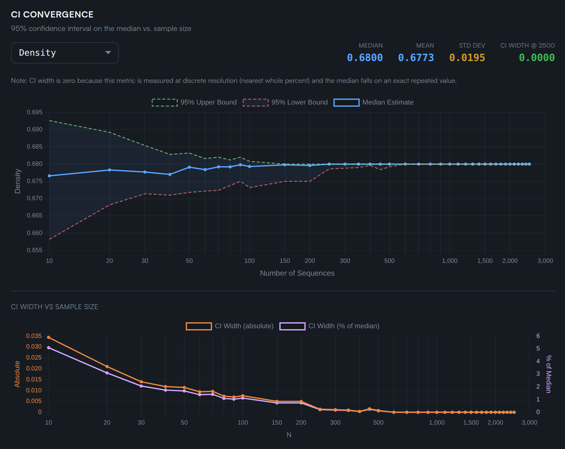
A single number means nothing without a confidence interval. We use distribution-free order statistics to bound the true median of each metric — no distributional assumptions required.
The idea is clean: sort your n observations and pick the k-th and (n−k+1)-th smallest values. The probability that the true population median lies between them is determined entirely by the binomial distribution — not by any assumption about the shape of the underlying distribution.
The charts below show how the 95% CI narrows as we add more sequences. For low-variance metrics like density, 100 sequences is often sufficient. For higher-variance metrics like fissure area, we need substantially more.
03
Not All Metrics Are Equal
The coefficient of variation (CV = std / mean) reveals which metrics have inherently higher variance and which are stable enough to detect small policy improvements.
We track a number of metrics beyond the primary KPIs for detailed monitoring of how any update to the packing agent affects the behavior and performance of the entire system. The chart below ranks them by CV.
Fissure metrics have CVs of 0.5+ — the standard deviation is half the mean. A single sequence can't tell you much about fissure quality — you need many runs to separate signal from variance. By contrast, density has a CV of just 0.037 — the wall volume fraction is tightly constrained by the geometry of the task, so it's extremely stable across sequences.
This asymmetry matters: an agent change that looks like it improved fissures on 5 sequences might just be sampling variance.
The practical implication: when we make algorithmic changes targeting higher-variance metrics (like fissure area), we need 3–5x more evaluation sequences than when targeting stable metrics (like density) to achieve the same statistical power for detecting improvements.
04
Why Random Shuffling Is Misleading
A tempting shortcut for generating more evaluation data: randomly shuffle the box sequence. But real warehouse sequences have local structure that shuffling destroys — and this can silently bias your evaluator.
We looked at real-world package sequence data with over 500K total boxes, using a sliding 25-box window. For each window, we computed simple aggregates: how many small boxes? How many heavy ones? Total weight? We then compared these distributions between the original ordered sequences and uniformly shuffled copies.
Real-world sequences are rarely random walks. WMS batching logic releases orders in waves (e.g. all small electronics first); supplier packaging means consecutive boxes from the same vendor share similar dimensions; and physical constraints often group heavy items together. These effects create runs of similar boxes that shuffling destroys.
The result is striking. Shuffling preserves global rates (the means are identical) but collapses local variance by ~1.4x. An agent evaluated on shuffled data faces a fundamentally different — and easier — sub-sequence distribution than one evaluated on real data.
| Property | Description | Ordered Std | Shuffled Std | Std Ratio |
|---|---|---|---|---|
| Small Box Count | Count of small boxes (all dimensions < 300mm) | 2.85 | 1.98 | 1.44x |
| Large Box Count | Count of large boxes (any dimension > 600mm) | 2.85 | 2.00 | 1.42x |
| Heavy Box Count | Count of heavy boxes (weight > 30 lbs) | 2.62 | 1.86 | 1.41x |
| Light Box Count | Count of light boxes (weight < 10 lbs) | 4.73 | 3.49 | 1.36x |
| Flat Box Count | Count of flat boxes (smallest dim / largest dim < 0.3) | 2.49 | 1.75 | 1.43x |
| Total Weight | Total weight (lbs) of boxes in the window | 113.08 | 83.24 | 1.36x |
| Total Volume | Total volume (m^3) of boxes in the window | 0.33 | 0.23 | 1.39x |
Small Box Count
Count of small boxes (all dimensions < 300mm).
1.44x std ratio — Small boxes cluster: more all-small and no-small windows than chance.
Large Box Count
Count of large boxes (any dimension > 600mm).
1.42x std ratio — Large boxes group consecutively in real ordering.
Heavy Box Count
Count of heavy boxes (weight > 30 lbs).
1.41x std ratio — Heavy boxes bunch up rather than being evenly distributed.
Total Weight
Total weight (lbs) of boxes in the window.
1.36x std ratio — Total window weight varies more in real ordering.
05
No Free Lunch, But a Good Pareto Curve
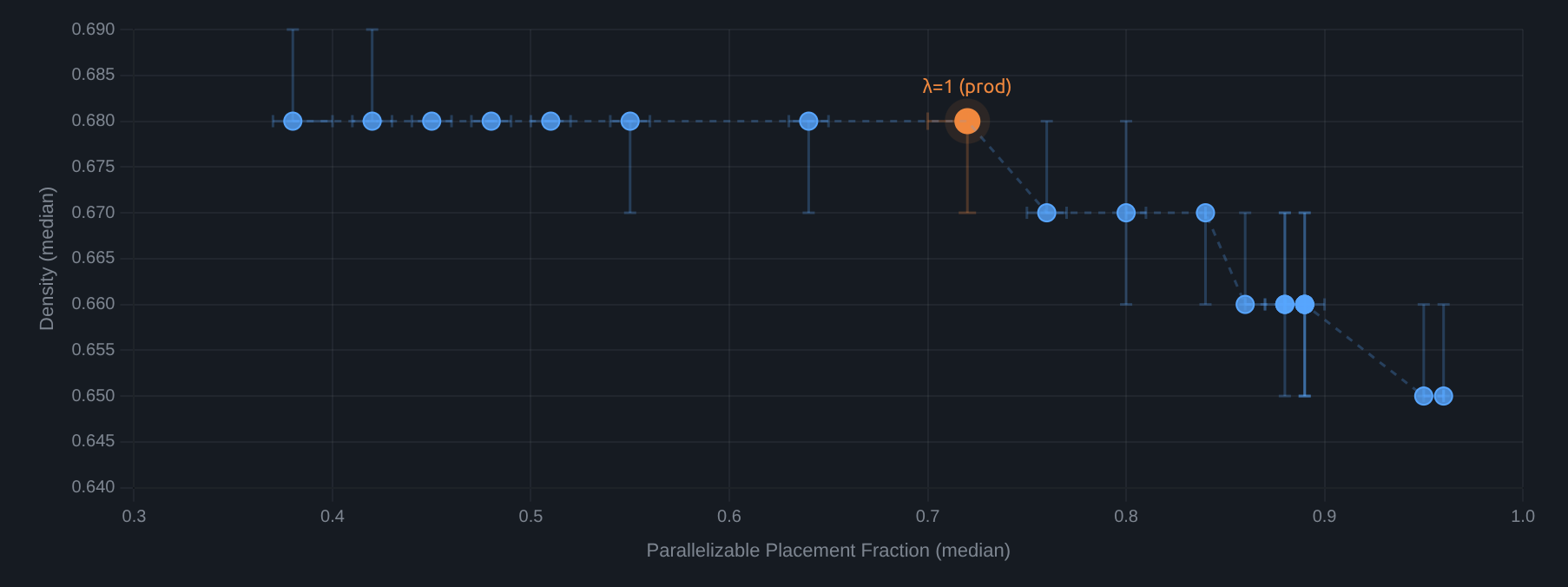
Foresight jointly optimizes for multiple objectives. There's no escaping the tradeoff — but we can design models to protect the metrics that matter most while accepting cost elsewhere.
The parallelism objective encourages placing boxes in positions where a second robot arm can work simultaneously. Higher parallelism means higher throughput — but it constrains placement choices, potentially affecting other metrics.
By sweeping the weight λ on the parallelism objective, we trace out the Pareto frontier. The key insight: the Foresight packing agent preserves density even as parallelism increases. In the regime we care about (λ ≤ 1), going from 38% to 72% parallelizable placements costs only 0.00–0.01 in density — the curve is essentially flat. The agent has learned to find placements that are simultaneously dense and parallelizable. Only at extreme parallelism targets (λ » 1) does density begin to drop.
Not all metrics are so easily maintained. Tilt stays remarkably flat across the entire frontier, but fissures increase meaningfully. Density is the metric we've specifically designed to protect; fissures are where the tradeoff cost surfaces.
06
Robustness Under Perception Noise
In production, Foresight doesn't see the world perfectly. Boxes have uncertain dimensions, positions drift, and sensor noise is ever-present. A packing agent that only works under perfect perception is useless.
We inject controlled noise into the physics simulation — perturbing observed box positions, dimensions, orientations, and weights — to measure how gracefully each metric degrades. Four noise axes, three magnitudes each, three key metrics tracked.
| Noise Axis | Max Level | Density | Tilt | Fissures |
|---|---|---|---|---|
| Position | ±3 cm | -0.02 (-2.9%) | +1.35 (+58.4%) | +0.11 (+14.5%) |
| Size | ±3 cm | -0.01 (-1.5%) | +0.42 (+18.2%) | +0.01 (+1.3%) |
| Rotation | ±3 deg | -0.03 (-4.4%) | +0.89 (+38.5%) | +0.04 (+5.3%) |
| Weight | ±15 % | +0.00 (+0.0%) | +0.07 (+3.0%) | -0.02 (-2.6%) |
Density is remarkably resilient. Even at ±3cm position noise — a substantial perturbation — median density drops only from 0.68 to 0.66 (3%). Size noise at ±3cm costs just 1.5%. Weight noise up to ±15% has effectively zero impact on density.
Tilt is the most sensitive metric. Position noise at ±3cm increases mean tilt from 2.31° to 3.66° (+58%). This makes physical sense: when boxes are placed slightly off from where the agent intended, they settle at larger angles.
Fissures stay controlled. The worst case (position ±3cm) increases fissure sum by ~14%. Weight noise has essentially no effect on any metric, confirming that the agent is robust to moderate relative error in weight.
These results give us confidence that Foresight's approach degrades gracefully rather than catastrophically under real-world sensing conditions.
Part II
Execution Intelligence
Part I evaluated how Foresight plans — density, stability, parallelism, and the tradeoffs between them. These sections show what happens when those plans meet the real world: dual-arm coordination, predictive pipelining, and what the system does when its predictions are wrong.
07
Predictive Pipelining
Predictive pipelining lets both robot arms operate concurrently — one arm picks while the other places, with no idle waiting. In production, 65% of placement decisions plan against predicted future state rather than waiting for fresh observations. This is how dual-arm throughput stays high.
In a serial system, each arm waits for the other to complete before planning its next move. Predictive pipelining eliminates this wait. When Arm A picks a box, the system predicts where that box will land — and critically, how that placement will affect the surrounding neighborhood. Placements use force-controlled tight-packing motions that push boxes into contact with their neighbors, so a single placement can shift, compress, or tilt adjacent boxes.
The system predicts this neighborhood effect, and Arm B plans its next action against this predicted world state — both arms plan concurrently rather than taking turns. Before execution, the planned trajectory is validated against the system's current estimate of the world.
The following metrics come from the last 5,000 boxes from production, analyzed from execution audit logs.
Two-thirds of all placement decisions plan against predicted in-flight state. Pipelining also meaningfully constrains the search space: 29% of candidate placements are filtered out because the predicted uncertainty in their placement neighborhood is too high — a nearby box is still in flight, and its effect on surrounding boxes hasn't settled yet. This isn't wasted computation — it's the system proactively avoiding regions of the trailer where the outcome is uncertain.
To isolate the throughput impact of parallelism, we ran an apples-to-apples comparison in simulation: the same ~1,500-box workload with parallel arm motion enabled vs. disabled.
Dual-Arm Throughput: Parallel vs. Serial
Simulation benchmark — same ~1,500-box workload, same config. Only difference: parallel arm motion enabled vs. disabled.
08
When Predictions Are Wrong
When the prediction is wrong — the world changes significantly between planning and execution — the trajectory fails validation. This happens in only 0.6% of cases. When it does, the system automatically replans and recovers 80% of the time.
Before executing any pipelined trajectory, the system validates it against its current estimate of the world — not the predicted one it was planned against. Small changes are absorbed naturally; the validation catches cases where the world has changed enough to warrant re-evaluation. When that happens, the system replans against the updated state. This validation step adds negligible latency — it is a read-only sensor query. If replanning also fails, the box is returned to its pick location for a retry on the next cycle. No crash, no damage — just a small throughput hiccup.
Net effect: predictive pipelining delivers a 33% throughput improvement with a <0.2% effective failure rate — 9 unrecovered mismatches out of 5,000 placement searches. The CI bands in Section 02 comfortably contain this noise.
Conclusion
Systematic Evaluation at Production Scale
These evaluations — from offline packing benchmarks to real-time pipelining metrics — represent one snapshot of a system under continuous development. Every improvement to Foresight's planning, every change to our reward structure, every refinement to our execution pipeline gets validated through the methodology described above: thousands of sequences, distribution-free confidence intervals, multi-objective Pareto analysis, and production telemetry from real robot sessions. High performance under nominal conditions, graceful degradation under perturbation — that's what separates a research system from a production system.
Open Evaluation
Foresight Packing Challenge launches March 23
We're opening this problem to the community with a turn-based API where your agent receives boxes one at a time and decides where to place them, with a full physics simulation in the backend. Let's pack!
Learn more about the Foresight Packing ChallengeDexterity — Inside Foresight — March 2026